Mutation-selection balance

In finite populations, new alleles are introduced continuously by mutation and their abundance subject to genetic drift. If their effects are not neutral, however, selection acts as well. In the steady state, a balance between drift and selection sets in and determines the spectrum of allele frequencies. The full script for this example can be found in the examples folder, in mutation_selection_balance_lowd.py.

First, after loading all necessary modules, we set the parameters as usual and create the population class:

N = 500                             # population size
L = 4                               # number of loci
s = np.linspace(-0.2 ,0.7, L) / N   # additive selection coefficients for L loci, scaled to N
mu = 0.4 / N                        # mutation rate, scaled to N
r = 5.0 / N                         # recombination rate for each interval between loci.

pop = h.haploid_lowd(L)             # produce an instance of haploid_lowd with L loci

Note that selection coefficients go from negative to positive across the L sites. We set the fitness landscape of the population:

pop.set_fitness_additive(0.5 * s)

Note

FFPopSim models fitness landscape in a +/- rather than 0/1 basis, hence the factor 0.5

We set the mutation/recombination rates, using a full multiple-crossover model:

pop.set_mutation_rates(mu)          # mutation rate
pop.set_recombination_rates(r)      # recombination rate (CROSSOVERS model by default)

We fix the carrying capacity and initialize the population with wildtypes only:

pop.carrying_capacity = N           # set the population size
pop.set_genotypes([0], [N])         # wildtype individuals, that is ----

Now we can start to evolve the population. We first let it equilibrate towards the steady-state:

pop.evolve(10 * N)                  # run for 10N generations to equilibrate

and we start to record the allele frequencies from now on:

for ii in range(nsamples):
    pop.evolve(0.1 * N)             # N / 10 generations between successive samples

    # get allele frequencies
    allele_frequencies[ii,:] = pop.get_allele_frequencies()

Finally, we histogram and plot the spectra of the single sites separately, since they have a different fitness coefficient:

for locus in range(L):

    y,x = np.histogram(allele_frequencies[:,locus], bins=af_bins, density='True')

    plt.plot(bin_centers, y, ...)

The result of the plot, compared to diffusion theory, is shown here below.

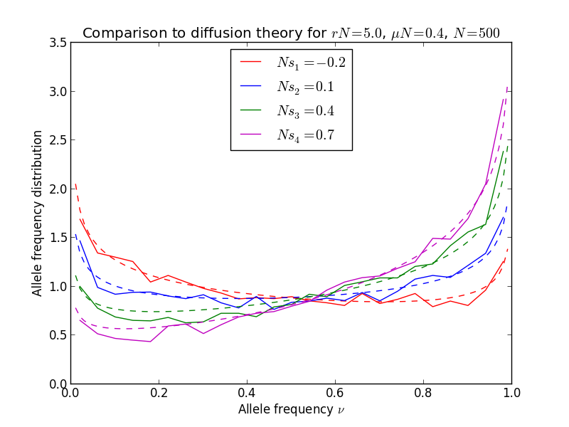
It fits the simulations quite well indeed; note the accumulation of alleles close to the boundaries. Note also that \(rN \gg 1\), hence the sites are essentially uncoupled.